WindowsInterfaces

To analyze the speed, bandwidth usage, and traffic handled by the network interfaces supported by a target server/application over time, pick the WindowInterfaces option from the Subsystem list. When this is done, Figure 1 will appear.

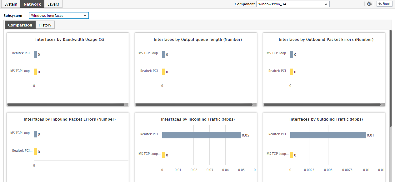
Figure 1 : The WindowInterfaces dashboard

1. Using the dial graphs and digital displays available in this dashboard, you can receive quick updates on current anomalies pertaining to the network interfaces supported by the target Windows-based component. Besides knowing what went wrong, you will also be able to identify which network interface has been affected, with the help of the dial/digital graphs displayed here.
2. Below the dial/digital displays, you will find the Comparison tab page, which provides a default collection of comparison bar charts, each of which compares the performance of the network interfaces in a specific performing sphere. Using these graphs, you can not only isolate performance anomalies, but also identify those network interfaces that are contributing to such anomalies.

3. Let us now refocus on the Comparison tab page. To view a comparison graph clearly, click on it; this will enlarge the graph as depicted by Figure 2.

   

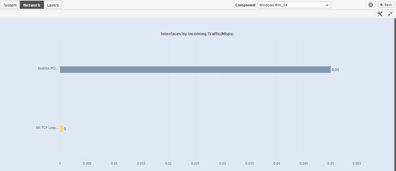
   Figure 2 : An enlarged comparison graph in the WindowsInterfaces dashboard

4. By default, the enlarged comparison graph will reveal only the top-10 network interfaces in a specific performance area. You can, if need be, view all the network interfaces supported by the target component, or only a few best/worst players in a performance area, in the enlarged mode. For this, select the relevant option from the Show list in the Settings option.

5. For deeper insights into the historical performance of the network interfaces, use the History tab page. By default, the History tab page of Figure 3 displays measure graphs depicting the time-of-day variations in the performance of the network interfaces supported by the target host. By default, these measure graphs are plotted for the last 24 hours. To analyze performance over a wider time range, click the Timeline link at the right, top corner of the History tab page to change the graph timeline.

   

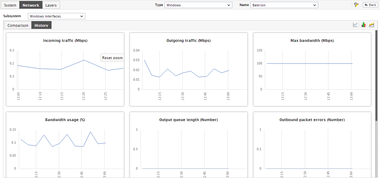
   Figure 3 : The History tab page of the WindowsInterfaces dashboard

6. You can enlarge a measure graph by clicking on it, and thus view it more clearly (see Figure 3).

   

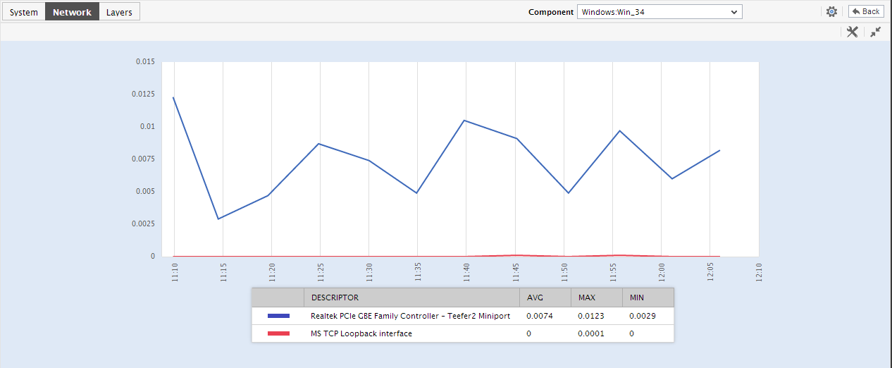
   Figure 4 : An enlarged measure graph in the History tab page of the WindowsInterfaces dashboard

7. Like the comparison graphs, the enlarged measure graphs also, by default, plot the values of the top-10 network interfaces supported by the device. Accordingly, the top-10 option is by default chosen from the Show list. To zoom into the performance of only a few of the top players / weak players in that performance area, pick a top-n or last-n option from the Show list of the Settings option.
8. Besides enabling you to identify the best/worst performers in a chosen performance arena, the enlarged graph also enables you to assess performance of network interfaces across broader time periods - for this, you will have to select a different Timeline for the enlarged graph.

9. To view the percentage of time during the last 24 hours for which a network interface was affected by issues, click on the icon at the right, top corner of Figure 4.

   

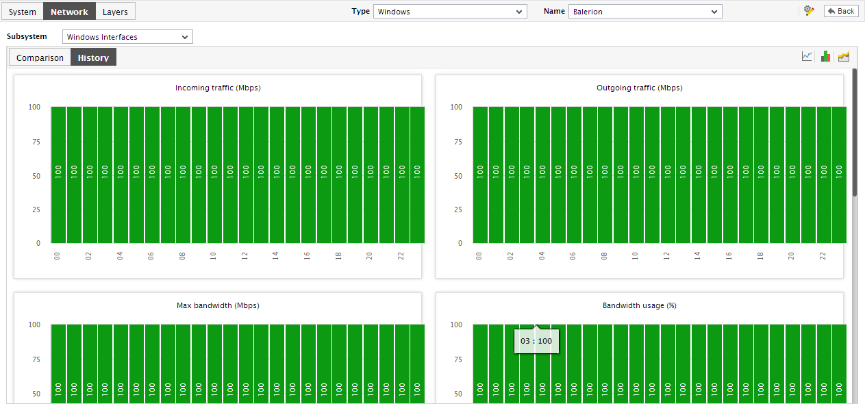
   Figure 5 : Summary graphs in the History tab page of the WindowsInterfaces dashboard

10. Using the graphs in Figure 5, you can effectively perform service level audits and detect when and what type of network issues caused the agreed-upon service levels to be compromised.

11. Similarly, click on the icon at the right, top corner of the History tab page in Figure 6 to view and analyze the past trends in network interface performance. By default, the trend graphs will pertain to the last 24 hours.

    

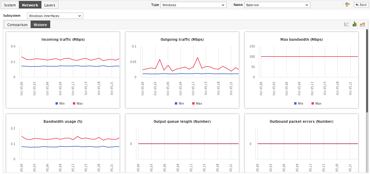
    Figure 6 : The Trend graphs in the dashboard of the Network subsystem

12. Using these trend graphs, you can determine when the performance of network interfaces peaked and when it hit rock bottom - this way, you can easily infer how network interface health has varied during the last 24 hours, and thus receive a heads-up on potential interface-related anomalies.
13. Besides the above, you can instantly change the timeline of the measure/summary/trend graphs in the History tab page by clicking on the Timeline link at the right, top corner of the tab page. To change the timeline of a single graph on the other hand, click on the graph to enlarge it, and then proceed to change its timeline. In the enlarged mode, you can even change the graph dimension (3d / 2d).
14. Also, an enlarged summary/trend graph allows you to alter the graph Duration - i.e., view the daily or monthly summary/trend information, instead of the default hourly data in the graphs.

15. Moreover, by default, the trend graphs in the History tab page plot the minimum and maximum values of a measure during the given timeline. In enlarged trend graphs, you can change the Graph type so that the average values or sum of trend values are plotted in the trend graphs instead.

    Note:

    In case of descriptor-based tests, the Summary and Trend graphs displayed in the History tab page typically plot the values for a single descriptor alone. To view the graph for another descriptor, pick a descriptor from the drop-down list made available above the corresponding summary/trend graph.

16. At any point in time, you can switch to the measure graphs by clicking on the button.