Proactive Observability – Predictive Analytics Models and Algorithms for IT Systems and Metrics

Predictive Analytics Models and Algorithms are an important component of eG Enterprise’s AIOps engine for proactive observability. eG Enterprise collects and analyses metrics, events, logs and traces and the data including real usage data is used to make intelligent predictions to forecast future system behavior and IT resource metric levels.

Today, I’ll familiarize you with some of the models and algorithms used within AIOps platforms such as eG Enterprise and how you can access intelligent metric forecasting for your IT systems.

Forecasting Use Cases

Many eG Enteprise customers leverage our forecasting analytics for a range of uses including:

• Capacity Planning – Forecast disk usage, memory, or node count to plan scaling ahead of time
• Latency Prediction – Anticipate increases in request latency before SLAs (service Level Agreements) are breached
• Traffic Forecasting – Predict incoming requests to auto-scale pods or services
• Error Rate Forecasting – Spot rising trends in error logs or HTTP 5xxs before a failure

Time Series Forecasting – An Overview

Time series forecasting is the process of predicting future values based on previously observed data points collected over time. It identifies patterns such as trends, seasonality, or cycles to model and forecast future outcomes. Commonly used in finance, operations, and weather prediction, it helps organizations plan resources, manage risks, and make data-driven decisions.

Components of Time Series Forecasting Models

The core components of a time series forecasting model can include:

• Trend – Long-term increase or decrease in the data.
• Seasonality – Regular, repeating patterns or cycles over fixed periods (e.g., weekly, monthly).
• Cyclicality – Irregular, non-fixed patterns related to economic or external cycles.
• Level – Baseline value around which variations occur.
• Noise (Residuals) – Random or irregular fluctuations not explained by other components.

Time Series Analysis vs Time Series Forecasting – What is the difference?

Time series analysis involves examining data points collected or recorded at specific time intervals to identify patterns, trends, and seasonal effects. It helps understand the underlying structure of the data and detect any changes over time. In contrast, time series forecasting uses historical data to make predictions about future events. While analysis focuses on interpreting past behavior, forecasting aims to estimate what will happen next. Together, they provide valuable insights for decision-making by combining historical understanding with future outlooks based on temporal patterns in the data.

Useful Forecasting Models

Autoregressive (AR) models

An autoregressive forecasting model predicts future values in a time series by using previous observations as input. It assumes that past values have a direct influence on current and future outcomes. The model analyzes how previous data points relate to each other over time to identify patterns, making it useful for short-term, linear, and stable data trends. AR models are the fundamental building blocks in more complex models such as ARIMA.

Polynomial regression for forecasting fits a curved line (polynomial function) to time series data, capturing non-linear trends. It models relationships using higher-degree terms (e.g., quadratic, cubic) beyond linear ones (straight lines) to predict future values based on past observations.

ARIMA – Autoregressive Integrated Moving Average

ARIMA forecasting predicts by analyzing past trends, seasonality, and irregularities, selecting optimal model parameters, and generating forecasts. It consists of 3 components:

1. AutoRegressive (AR) Component: models the relationship between the current observation and its lagged values. Past values are used to predict and forecast future values.
2. Integrated (I) Component: This component involves differencing the time series data to make it stationary. A stationary time series is one whose statistical properties such as mean, variance, and autocovariance remain constant over time. Differencing helps remove trends and seasonality, making the data more amenable to modeling.
3. Moving Average (MA) Component: This component models the relationship between the current observation and a linear combination of past forecast errors. It captures short-term irregularities or noise in the data i.e. it uses past forecasting errors to improve predictions.

STL (Seasonal-Trend decomposition using Loess)

STL is a time series decomposition algorithm that separates a series into three components – Seasonal, Trend and Remainder (Residual). STL forecasting is effective for time series with complex seasonal patterns and irregular trends. It decomposes time series data into trend, seasonal, and residual components using Loess smoothing. It enables the extraction of underlying patterns and facilitates forecasting by modeling the trend, seasonality, and remainder separately.

STL uses LOESS (a non-parametric local regression) to smooth and separate these components. Unlike classical decomposition, STL is flexible and robust to outliers.

STL strengths:

• Works with both short and long seasonal periods
• Handles changing seasonality
• Robust against outliers
• Suitable for both additive and multiplicative models

STL is often used to pre-process data for ARIMA, STL analysis is used to enable forecasting via ARIMA. STL is also good at anomaly detection on historical data sets.

Frequency Domain Forecasting

Frequency Domain Forecasting involves analyzing time series data in the frequency domain rather than the time domain. It’s like looking at a song’s melody in terms of its harmonies and rhythms rather than the sequence of notes/sounds over time. In this model, techniques such as Fourier analysis is used to decompose the time series into its constituent frequencies. This helps in identifying periodic patterns, seasonality, and trends more clearly, making it easier to forecast based on the underlying frequency components.

Frequency Domain Analysis is often used alongside or as a pre-processing step for time domain modelling using algorithms such as ARIMA.

ARIMA within eG Enterprise v7.5

From version 7.5 a customized ARIMA model is the default used for forecasting and predictive analytics within eG Enterprise. Additional algorithms and predictive analytics models that eG Enterprise support include options for:

• Frequency Domain
• Polynomial Autoregression
• STL

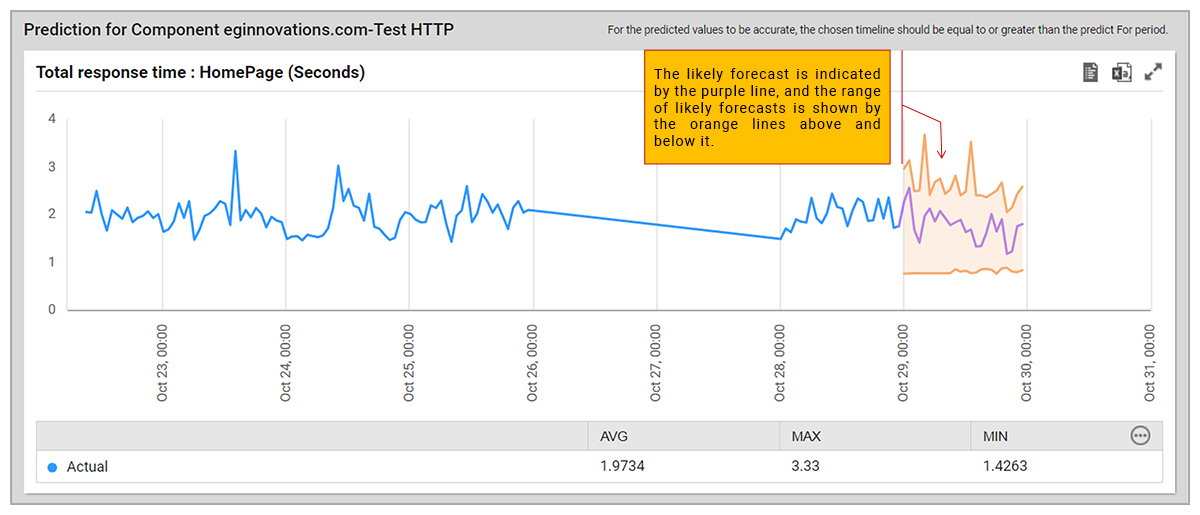
Forecasts are now also displayed with ranges by default.

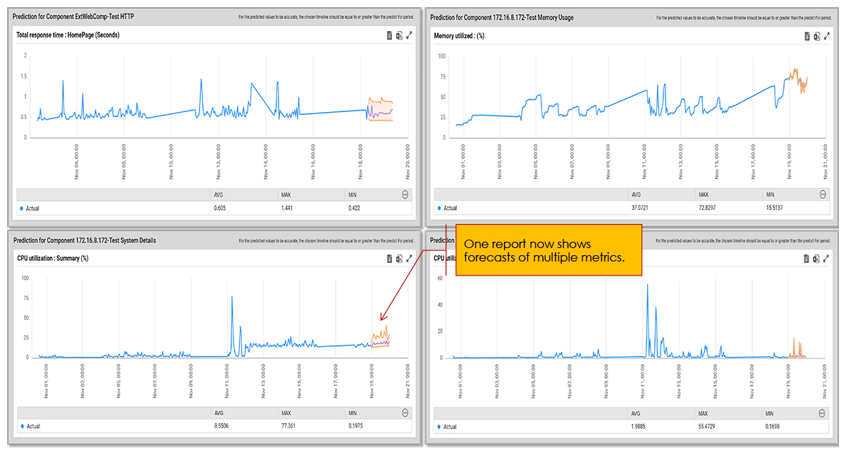
In previous versions you could only forecast one measure at a time. Now, with eG Enterprise v7.5, you can also add multiple measures for forecasting.

Forecasting Reports within eG Enterprise v7.5

It’s easy to access ready-built predictive analytics reports in eG Enterprise v7.5. From the “Reporter” tab in the main console select “Prediction Analysis” under the Reports section by function.